
Home | Biodata | Biography | Photo Gallery | Publications | Tributes
Iconometry
| |
Home | Biodata | Biography | Photo Gallery | Publications | Tributes Iconometry |
|
Introduction
Principal component and factor analytic techniques, which have been applied in such varied fields as psychology, education, anthropology, music and literature, (Jeffers, 1967) can be extended to an even wider range of problems and subjects. Applied to the study of South Indian sculptures of the eighth century A.D., they may contribute to the solution of major problems in art history, such as the dating of sculptures in a major temple.
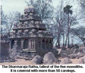
In the Madras region of Southern India the earliest surviving sculptures belong to the seventh and eighth centuries A.D. The region was ruled by kings belonging to the Pallava dynasty whose capital city was Kanchipuram and whose chief port was Mahabalipuram or Mamallapuram. The earliest surviving structural temples belong to the period of Rajasimha, who ruled from Kanchipuram around 700 A.D.; one of his surviving temples is the Kailasanatha temple at Kanchipuram (Srinivasan, 1972). Although the earlier shrines are in hard rock, the carvings of the Kailasanatha temple are in sandstone. At the beginning of this century, most of these carvings were reported by Alexander Rea (1909) of the Archaeological Survey of India to be covered with plaster. The recent removal of this plaster covering on many of the carvings, has exposed a marvelous collection of eighth century sculptures. The carvings illustrated in this article, being among those rediscovered, have not appeared in any major work on Indian art.
In this study of iconometry, we have measured point-to-point distances for about forty carvings of the Kailasanatha temple (Longhurst, 1930), and we have also - by use of a large computer - performed a multivariate analysis of the data.
Such a study of iconometric measurements will prove generally useful in dating sculptures, in restoration work, in checking whether any of the known canons of iconometry were followed by the sculptors, and for hypothesizing about the number of sculptors who executed the work, as Guralnick (1976, 1978) did in her pioneering application of statistical and computer methods to the study of Greek sculptures. In this approach, art historians do not usually depend on actual measurements to compare the styles of different sculptures, but rather depend largely on visual subjective impressions. The objective method of studying the similarity between Indian sculptures, introduced in this study, will reveal special features that have been missed by earlier scholars. In dating sculptures, the average values of the iconometric features of different periods and regions will be useful, but we shall not take up that problem in this paper. To restorers, especially when these values differ considerably from canonical proportions, the average measurements for different types of images will also be of value. Using a technique called cluster analysis one can find out whether a given carving is closely similar to a given set of canonical proportions. These problems are discussed elsewhere (Siromoney, Bagavandas and Govindaraju, 1979).
In this paper we shall consider only the application of component and factor analysis techniques to the study of iconometric measurements of carvings of Kailasanatha temple at Kanchipuram.
Because these sculptures are carved in a variety of postures it is difficult to get meaningful measurements common to all of them. This article is illustrated with pictures of a drummer, playing on two vertical drums, who is looking away at a dancer, whose dance he accompanies.
A multiple-armed figure of a dancer is the dancing Siva, the Lord of the Dance. In some figures a deliberate foreshortening of the arm is employed by the sculptors who do not have enough material to work with. With figures represented in such a diversity of stances we have to limit ourselves to measuring only a small number of features. Furthermore unlike human subjects, for a given sculpture permits only certain measurements, for instance, one can take both the standing height and the sitting height of any human subject but this certainly is not possible for a single sculpture depicted in a specific stance. To compare a large number of sculptures we have therefore confined ourselves, in this paper, to ten facial measurements.
Principal component analysis is applied to facial measurements and the results are presented in the Section Analysis of facial measurements. In the Section thereafter, the facial proportions are studied through component analysis and factor analysis, and different meaningful factors are extracted.
| 
|
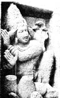
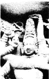
| Fig. 1. A drummer playing on two vertical drums with his face turned toward a dancer. He is represented on the upper portion of the niche. The lower portion, not shown in the picture, contains a flutist and a cymbalist who also accompany the dancer. On the headdress of the drummer is an axe-head, an emblem of Siva, who is the dancer shown in an adjoining niche. The three-headed cobra seen in the picture is also associated with Siva. | Fig. 2. The dancing Siva, shown with eight arms. In one of his right hands he holds a small hour-glass-shaped drum. |
| 
|
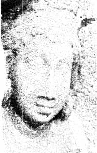
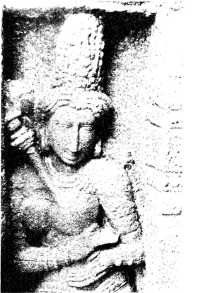
| Fig. 3. The goddess Parvati. This beautiful carving is found in a niche along with Siva on the northern side of the main tower. | Fig. 4. A maid holding a fly-whisk or chauri. Her nose is extraordinarily long and the distance from nose-to-chin is unusually short. According to the Indian canons of iconometry, the nose should be one-third the face length. |
Analysis of facial measurements
For this analysis, facial measurements were obtained from 39 undamaged relief sculptures representing gods and goddesses, male worshippers, and female attendants. All the sculptures are found on the outer walls of the main sanctum and in the side shrines of the main tower. Not included are figures from the small shrines forming the enclosure since most of them have not been cleared of the thick plaster coating. Also excluded from the study are the representations of dwarfs, doorkeepers, asuras (giants) and ardhanarisvara with each half representing a different deity, one male and the other female. One of the authors, using anthropometric instruments, took measurements for ten variables from each sculpture. These are defined in anthropometric terminology (Singh and Bhasin, 1968) as follows:
| NOSELENG | the nose-length
 the straight distance between the root of the nose and subnasal. the straight distance between the root of the nose and subnasal. |
| NOSEBRTH | the nose-breadth
the straight distance between most laterally placed points on the
nasal wings. |
| LIPLENGT | the lip-length the straight distance between the two corners of the mouth. |
| LIPBRETH | the lip-breadth
the straight distance between labral superior and
labral inferior. |
| FACEBRTH | the face-breadth
the straight distance between the two tragia. |
| EYELENGT | the eye-length the straight distance between the internal and the external corners of the eye. |
| EYEBRETH | the eye-breadth
the maximum distance between the eyelids. |
| NOSTOCHN | nose-to-chin the straight distance between subnasal
and gnathion. |
| FACELENG | the face .length
the straight distance between hairline or crown base
and gnathion. |
| MFACLENG | the morphological face-length
the straight distance, between the root of the nose and the gnathion. |
Table 1 gives a summary of data for the ten variables. A number of interesting observations may be made from the mean values of the variables. According to the surviving canons of Indian iconometry (Banerjea, 1956), the nose-length and the distance from nose to chin must be equal. From the table we find that the sculptors of the Pallava dynasty who built the Kailasanatha temple had a preference for long noses and a short nose-to-chin distance. The unusual length of these Pallava noses, overlooked by art historians, seems to be a peculiar characteristic of the period of King Rajasimha Pallava, who built the temple.
Table 2 gives the coefficients of correlation between each of the ten facial measurements. All the coefficients are positive and significant at 1% level. As a note of caution, we wish to point out that there are no grounds to assume that the 39 sculptures form a random sample from a population of Pallava sculptures of Kanchipuram belonging to circa 700 A.D. All we can say is that each sculpture is a priceless piece of art and that we have a sample of 39 pieces. One comes across this kind of problem quite often in the field of archaeology.
It is clear, therefore, that the ten different measurements that we have taken are not independent, but highly related to each other. The next question then is, can we reduce the number of measurements that can explain the variability between the different sculptures? Instead of ten different measurements, can two or three measurements of a different kind explain the variability? These questions can be answered by using the techniques of principal component analysis (PCA). Given a set of variables and their correlation matrix, a PCA can reduce the number of correlated variables to a smaller number of independent variables or of principal components, which are linear combinations of statistical variables having special properties in terms of variances (Anderson, 1972). Transforming a given set of variables to a set of principal components amounts to a rotation of coordinate axes to a new coordinate system. The method of PCA is used to find linear combinations with large variances.
The first principal component, which accounts for 90% variability, is a linear combination of the ten variables. The different weights of these variables that contribute to the first principal component are given in table 3.Giving more or less equal weighting to all the variables, it may be regarded as a general index of size of the sculptures.
Table 1
Summary of data for facial measurements (cm)
| Variable | Minimum | Mean | Maximum | Standard deviation |
| NOSELENG | 3.1 | 4.900 | 7.6 | 0.990 |
| NOSEBRTH | 2.0 | 3.282 | 6.0 | 0.814 |
| LIPLENGT | 2.6 | 3.997 | 7.0 | 0.981 |
| LIPBRETH | 1.2 | 1.592 | 2.5 | 0.290 |
| FACEBRTH | 7.1 | 10.192 | 15.9 | 2.086 |
| EYELENGT | 1.9 | 3.095 | 5.3 | 0.695 |
| EYEBRETH | 0.4 | 0.718 | 1.3 | 0.215 |
| NOSTOCHN | 2.2 | 3.264 | 5.4 | 0.807 |
| FACELENG | 7.5 | 10.951 | 17.5 | 2.283 |
| MFACLENG | 5.4 | 8.182 | 12.9 | 1.725 |
|
Table 2 |
|||||||||
|
Coefficients of correlation between facial measurements |
|||||||||
| NOSELENG | |||||||||
| 0.938 | NOSEBRTH | ||||||||
| 0.989 | 0.933 | LIPLENGT | |||||||
| 0.862 | 0.869 | 0.833 | LIPBRETH | ||||||
| 0.951 | 0.946 | 0.917 | 0.849 | FACEBRTH | |||||
| 0.877 | 0.873 | 0.813 | 0.815 | 0.869 | EYELENGT | ||||
| 0.846 | 0.866 | 0.789 | 0.786 | 0.869 | 0.843 | EYEBRETH | |||
| 0.881 | 0.910 | 0.893 | 0.833 | 0.929 | 0.803 | 0.831 | NOSTOCHN | ||
| 0.979 | 0.957 | 0.917 | 0.895 | 0.963 | 0.892 | 0.864 | 0.930 | FACELENG | |
| 0.975 | 0.954 | 0.921 | 0.880 | 0.964 | 0.868 | 0.869 | 0.961 | 0.988 | MFACLENG |
Table 3
Weights for the first principal component of facial measurements
| Variables | Weights |
| NOSELENG | 0.323 |
| NOSEBRTH | 0.324 |
| LIPLENGT | 0.313 |
| LIPBRETH | 0.302 |
| FACEBRTH | 0.324 |
| EYELENGT | 0.303 |
| EYEBRETH | 0.300 |
| NOSTOCHN | 0.314 |
| FACELENG | 0.329 |
| MFACLENG | 0.329 |
Percentage of variability 90.29
Table 4
Summary of data for facial proportions in
angulas face-length is taken to be 12 angulas
| Variables | Minimum | Mean | Maximum | Standard deviation |
| NOSELENG | 4.80 | 5.377 | 5.87 | 0.244 |
| NOSEBRTH | 3.06 | 3.579 | 4.11 | 0.269 |
| LIPLENGT | 3.50 | 4.365 | 5.13 | 0.424 |
| LIPBRETH | 1.37 | 1.760 | 2.13 | 0.074 |
| FACEBRTH | 9.83 | 11.213 | 12.37 | 0.607 |
| EYELENGT | 2.71 | 3.395 | 4.38 | 0.359 |
| EYEBRETH | 0.55 | 0.780 | 1.07 | 0.126 |
| NOSTOCHN | 2.91 | 3.562 | 4.21 | 0.316 |
| MFACLENG | 8.39 | 8.965 | 9.65 | 0.291 |
One of the avowed aims of PCA is to reduce the number of variables to a smaller number of independent components which will explain a high proportion of the variability in the sample. Although we have succeeded in explaining 90% of the variability in terms of a single principal component, we also find that the first principal component is primarily an index of size. The question that arises naturally in this context is whether the same multivariate data can be described in terms of a smaller number of major factors if all the variables are made independent of size. We shall devote the next section to the discussion of such questions.
Analysis of facial proportions
One way of making the variables independent of size is to decide on a suitable variable and to convert the other variables as proportions with respect to the one chosen. From the correlation matrix of table 2 it is possible to find those variables that have high column totals. Face length and morphological face length are the variables which have the highest correlations with the others. On the basis of theoretical as well as practical considerations, one of these variables can be chosen for the purpose. There are sufficient reasons for choosing face length as the required variable for standardizing the remaining nine variables.
The Indian canons of iconometry follow a proportionate unit of measurement called the angula or finger-width, twelve of which make a face-length; we shall express all facial proportions in terms of the angula. To convert each variable to a proportion in angulas, we shall divide each variable by the corresponding face length and multiply it by 12. The nine facial proportions are given in table 4. For the proportions also we shall, for the sake of convenience, retain the corresponding variable names throughout this section.
According to the surviving canons of iconometry both nose-length and nose-to-chin are prescribed to be four angulas. In some texts there are occasional variations, but none allows long noses with an average of 5.37 angulas against the nose-to-chin value of 3.56 angulas, such as appear in table 4. There is, therefore, hardly any evidence from table 4 to support the theory that the sculptors of Kailasanatha temple followed any of the canons that have come down to us. In spite of the lack of randomness of our sample, the mean values of the different facial proportions would be estimates of the population values whether or not the sculptors consciously followed any canon of their own. If they did, then we have recovered the values of facial proportions and these are undoubtedly very different from any of the known canonical proportions. Mean values for different categories of sculptures would prove useful in restoration work.
Table 5
Coefficient of correlation between facial proportions
| NOSELENG | ||||||||
| 0.06 | NOSEBRTH | |||||||
| -0.041 | 0.491a | LIPLENGT | ||||||
| -0.166 | -0.121 | -0.050 | LIPBRETH | |||||
| 0.277 | 0.101 | 0.174 | 0.011 | FACEBRTH | ||||
| 0.125 | 0.026 | -0.016 | 0.060 | 0.171 | EYELENGT | |||
| 0.033 | 0.338a | 0.134 | -0.071 | 0.234 | 0.360a | EYEBRETH | ||
| -0.389a | 0.248 | 0.316a | -0.073 | 0.107 | -0.117 | 0.146 | NOSTOCHN | |
| 0.315a | 0.250 | 0.263 | -0.082 | 0.282 | -0.091 | 0.175 | 0.692b | MFACLENG |
Table 5 gives the coefficients of correlation between each of the nine facial proportions. These values are markedly different from the corresponding values given in table 2 obtained from facial measurements. The correlation coefficient between nose-length and eye-length for direct measurements is 0.88 in contrast to the insignificant value of 0.12 for the corresponding proportions. The special features of the sculptures of Kailasanatha temple
of gods and goddesses, male worshippers and female attendants are reflected in the correlation matrix of proportionate variables (table 5) and not in the correlation matrix of direct measurements (table 2). The addition of a few sculptures of dwarfs and doorkeepers to the sample would alter many values of table 5 since these figures have markedly short noses and round bulging eyes.
We find that nose-length is significantly correlated with morphological face-length and negatively correlated with nose-to-chin. The longer the nose, the shorter the length from nose-to-chin. Eye-length and eye-breadth are significantly correlated but nose-length and nose-breadth are not. The length of the lip is not significantly correlated with the nose length. Face-breadth as well as lip-breadth are not correlated with any variable. These and other peculiar characteristics of Rajasimha's period are brought out clearly by the correlation matrix of proportions and not by the correlation matrix of direct measurements.
We can apply PCA to the data of nine proportions to see whether there are significant principal components. If the first principal component explains a large proportion of variability it will be of great interest to the art historian, from the point of view of the relation of canonical texts to the actual measurements of sculptures.
There are differences of opinion among art historians as to whether canons of iconography and iconometry were used by the Pallava sculptors who built Kailasanatha temple. Some claim that these canons were used as early as A.D. 700 but other scholars set the date only around A.D. 800. This system of iconometry (Gopinatha Rao, 1920) prescribes different sets of proportions for the whole body from crown to foot, but for all the sets the facial proportions are practically the same. For any set of proportions for a given type of figure, all the facial measurements are given in angulas. According to Silparatnam (Devanathachari, 1961), a canon familiar to South Indian sculptors, the typical prescribed proportions for nose-length, nose-breadth, lip-length, lip-breadth and eye-length and eye-breadth are respectively, four, two, two, one and half, two and one angulas. These values are quite different from the average values (table 4) of the proportions of Kailasanatha sculptures. The main point, however, is that all the canonical proportions are expressible in terms of a single factor, the angula. Even if the proportions varied a little from canon to canon, the principle of expressing the proportions in terms of a single factor is common to all the Indian canons.
When the PCA is applied to the measurements of nine proportions, it is seen that the first principal component explains only 27% of the variation and the fifth principal component 10% of variation. Table 6 gives the percentage of variability accounted for by the principal components and the corresponding weights for the first five principal components. The fact that there are five factors, each of which accounts for a small variability from 10 to 27, would show clearly that they had not followed strictly any canons of the type with which we are familiar today. When the first two principal components cover a large proportion of variability one can graphically represent the data in terms of the two factors and look for natural clusters. Since our first two components account for only 45 of the variations, it is not possible to use this method to look for clusters, but a separate cluster analysis of data will be useful in finding out the carvings that are most similar to each other. Carvings which have a high degree of similarity may be attributed the same authorship. For such a study preliminary results are given elsewhere (Siromoney, Bagavandas and Govindaraju, 1979).
Although it may sometimes be possible to interpret the different principal components meaningfully, in our case it is a little difficult to interpret each component as representing an underlying factor. We shall therefore make certain assumptions about the underlying structure (Kendall and Stuart, 1968). Since the number of variables is nine it is legitimate to have a maximum of five factors (Anderson and Rubin, 1956). We shall assume that there are five main factors that go into the designing of a face: the nose-length, nose-breadth cum lip-length, eye-shape, lip-thickness, and face-width.
The morphological face-length and the nose-to-chin length shall be included in the nose-length factor. Since the face-length is fixed, the point at which the root of the nose is fixed automatically defines the morphological face-length. If the nose starts high up, then the morphological face-length is greater. The position of the tip of the nose, which defines the nose-to-chin measurement, therefore represents the nose-length and the positioning of the nose as reflected in the morphological face-length and the nose-to-chin measurement.
The nose-breadth cum lip-length factor reflects the way in which the nose is given its final shape in relation to the lip-length. If the sculptor had visualized a face with small lips (small lip length) then he would have adjusted the nose breadth accordingly. Similarly the design of the lips depended upon the nose-breadth. The eye-shape factor depends upon the eye-length and the eye-breadth. Because design of the face also depends upon the thickness of the lips and the width of the face, these are treated as factors.
For obtaining the factor loadings we give unity as trial value if a variable is included in a factor and zero otherwise. For the nose-length factor we give negative sign to the nose-to-chin variable. The factor loadings given in table 6 were obtained by extracting the factors in the following order: nose-breadth (20.0), eye-shape (15.5), nose-length (14.6), lip-breadth (11.1), and face-breadth (10.3). The numbers in parentheses refer to the corresponding percentages of variability explained by the factors. The five factors explain just over 71% of the variability.
In fashioning a face, the Indian sculptor would normally fix the nose-length first by drawing the middle portion of the nose and then add the nasal wings on its two sides and fix the nose-breadth. From the artist's point of view the first factor may alternatively be understood as the factor that comes first in designing the face and it need not be the factor which explains the largest proportion of variability in the sample.
If the first two main factors explained a large proportion of the variance one could graphically describe the data using two axes. Since the first two factors explain only about 35 percent of the variation we shall not use such a graphical method to locate groups. As mentioned earlier other methods of classification will have to be used to establish the existence of clusters.
Table 6
Weights for the first five principal components of facial proportions
| Variables | Principal components | ||||
| I | II | III | IV | V | |
| NOSELENG | 0.089 |
0.706
|
0.596 | 0.092 | 0.173 |
| NOSEBRTH | 0.655 | 0.016 |
0.259
|
0.441 | 0.276 |
| LIPLENGT | 0.638 | 0.153 |
0.150
|
0.258 | 0.500 |
| LIPBRETH |
0.189
|
0.080 |
0.340 |
0.688
|
0.517 |
| FACEBRTH | 0.443 |
0.477
|
0.150 | 0.362
|
0.180 |
| EYELENGT | 0.077 |
0.626
|
0.506
|
0.147
|
0.214
|
| EYEBRETH | 0.494 |
0.408
|
0.474
|
0.032 |
0.318
|
| NOSTOCHN | 0.702 | 0.540 | 0.011 | 0.292
|
0.313
|
| MFACLENG | 0.762 | 0.068 | 0.456 | 0.302
|
0.137
|
| Percentage of variability | 26.637 | 17.914 | 14.143 | 11.927 | 10.222 |
| Cumulative percentage of variability | 26.637 | 44.551 | 58.695 | 70.622 | 80.844 |
Table 7
Factor loadings for five factors of facial proportions
| Variables | Factors | ||||
| Nose-breadth | Eye-shape | Nose-length | Lip-breadth | Face-breadth | |
| NOSELENG |
0.021
|
0.101 | 0.975 |
0.068
|
0.022 |
| NOSEBRTH | 0.864 | 0.076 | 0.024 |
0.034
|
0.062
|
| LIPLENGT | 0.864 |
0.076
|
0.024
|
0.034 | 0.062 |
| LIPBRETH |
0.099
|
0.010 |
0.105
|
0.990 | 0.000 |
| FACEBRTH | 0.160 | 0.222 | 0.247 | 0.051 | 0.928 |
| EYELENGT | 0.005 | 0.836 | 0.019 | 0.054 |
0.025
|
| EYEBRETH | 0.273 | 0.790 |
0.019
|
0.054
|
0.025 |
| NOSTOCHN | 0.327 |
0.038
|
0.390
|
0.081
|
0.177 |
| MFACLENG | 0.297 | 0.000 | 0.368 |
0.014
|
0.155 |
| Percentage of variability | 20.0 | 15.5 | 14.6 | 11.1 | 10.3 |
| Cumulative percentage of variability | 20.0 | 35.5 | 50.1 | 61.2 | 71.5 |
Conclusion
The primary contribution of this study is advancing the use of computers to an additional field of art historical research. The study deals with an important body of material of the Pallava period from a temple which is one of the earliest structural temples of the Madras region in South India. There are no other comparable materials of this period. Further work on other important material of a later period is in progress. In addition to proportions, the distinctive costumes and jewellery (Lockwood, Siromoney and Dayanandan, 1974) depicted on the different categories will also be of value in restoration work.
Acknowledgement
The authors are thankful to the referees for their valuable comments, to Mr. L.K. Srinivasan, Superintending Archaeologist of the Archaeological Survey of India, for making it possible to take measurements of the valuable carvings, to Mr. R. Chandrasekaran for his valuable assistance in writing the FORTRAN program for IBM 370/155 computer, and to Mr. M. Chandrasekaran for valuable discussions.
References